Microsoft word - posters-d-f

Workshop on Agricultural Air Quality WATER9 – An Air Emission Model for Animal Feeding Operations –
Software for Both Field Agents and Comprehensive Scientific Research
M.E. Deerhake1, C.C. Allen2, and S. Nizich3 1RTI International, Research Triangle Park, NC 2RT Allen, Durham, NC 3U.S. Environmental Protection Agency, Research Triangle Park, NC Abstract
In response to the National Academy of Science's Board on Agriculture and Natural Resources and their
Ad Hoc Committee on Air Emissions from Animal Feeding Operations' (AFO) October 2003 final report
"Air emissions from Animal Feeding Operations: Current Knowledge Future Needs", RTI has supported
the U.S. Environmental Protection Agency in evaluating adaptations of the software program WATER9 as
a potential tool for use in providing scientifically sound estimates of air emissions from AFOs. The
committee recommended EPA and USDA use such model(s) with mass balance constraints for nitrogen-
containing compounds, methane, and hydrogen sulfide and adapt current or adopt new programs to fill gaps
in research to improve process-based models to increase the accuracy and simplicity of measuring and
predicting AFO emissions. In the 1990s, EPA contracted RTI to develop an emission model known as
WATER9 for other rulemaking efforts such as estimating volatile organic emissions from hazardous waste
management processes. Since that time, earlier versions of WATER9 have evolved to model other
emission sources, including biological treatment tanks and trickling filters, as well as gases that include
hydrogen sulfide. RTI has supported EPA in adapting WATER9 to predict AFO emissions by identifying
and collecting the necessary input data on poultry, beef, dairy, and swine for WATER9's adaptation and by
starting development of software to estimate ammonia, hydrogen sulfide, volatile organic and methane
emissions from housing, lagoons, pits, and spray fields, among other sources. Should EPA and USDA
adopt the model for this purpose, the current version of WATER9 for AFOs will be available in both a
comprehensive modeling package as well as a field package that would enable field agents to assist
growers with on-site nutrient management planning. This paper highlights the features of WATER9, its
benefits, validation, and flexibility.
The National Academy of Science's Committee on Air Emissions from Animal Feeding Operations in its 2003 final report AAir Emissions from Animal Feeding Operations: Current Knowledge, Future Needs@ stated that Aprocess-based modeling will help provide scientifically sound estimates of air emissions from AFOs for use in regulatory and [waste] management programs@ (NAS. 2003). The Committee recommended U.S. Environmental Protection Agency (EPA) and U.S. Department of Agriculture (USDA) use such model(s) with mass balance constraints for nitrogen-containing compounds, methane, and hydrogen sulfide; investigate the potential use of a process-based model to estimate mass emissions of odorous compounds; and adapt current or adopt new programs to fill gaps in research to improve process-based models to increase the accuracy and simplicity of measuring and predicting AFO emissions. The EPA, with support from RTI International, is evaluating WATER9, along with other process-based models, to address the NAS finding. WATER9 is a Windows-based computer program that estimates air emissions of individual waste constituents in wastewater collection, storage, treatment, and disposal processes. The model=s successful applications include the estimation of volatile organic emissions from hazardous waste management processes such as process vents, lagoons, and open storage tanks (see 40 CFR 264, subparts AA, BB, and CC). Since that time, WATER9 precursors have evolved to model a variety of emission sources, including biological treatment tanks, trickling filters, and cooling towers, as well as gases that include hydrogen sulfide. (See http://www.epa.gov/ttn/chief/software/water/index.html ) This paper presents WATER9's adaptation for use as a tool for AFOs. Workshop on Agricultural Air Quality Features
WATER9 for AFOs contains a variety of features to enable a comprehensive estimation of emissions from animal waste generation, storage, transfer, treatment, and disposal operations. The current version predicts emissions of ammonia, volatile organic compounds, Clean Air Act hazardous air pollutants, hydrogen sulfide, nitrogen, nitrogen oxides (NO and N2O), and carbon dioxide. It is capable of evaluating several livestock industries, including swine, poultry, beef, and dairy. Formal model features include the effects of surface area, temperature and wind, animal type and age, and design changes; a combination of removal mechanisms, including biodegradation, and chemical conversion and volatilization; pH effects; and effluent removal. Specific components have been designed for different types of animal confinement structures, feedlots, collection systems, waste piles, pits, impoundments, and land application units. The model can be used to predict the performance of crop uptake or air emission control devices. WATER9 uses proven correlations to calculate mass transfer coefficients and process unit input parameters to estimate emissions. WATER9's most important database is its extensive agricultural input information that includes waste generation rate by animal, waste characterization, properties of nitrogen, urea, uric acid and other waste constituents and by products. The user can adapt or add to these files. In addition, WATER9 features a Help file that describes, on command, AFO operations, advises on input values, animal and waste characterizations, case studies, and documents the model's validation. Active internet links are embedded in the Help file for the user, as well as a key word search function to expedite assistance. An added feature is the prediction of hydrogen sulfide bubble burst effects – an episodic condition that can threaten both the worker and the animal population. WATER9 reports in summary or detailed, unit-specific output, and it is amenable to designing new report formats.
Figure 1. WATER9 for AFOs offers a variety of menus for customizing emission modeling
(example screen shot).
Benefits
WATER9 for AFOs is more beneficial than routine use of emission factors because it computes unit specific and system-wide mass balance of waste constituents from point of generation through environmental release. It allows the user to calculate site-specific emissions, using the local AFO's design and operating parameters. Waste management unit emission estimates account not only for local meteorological conditions such as wind and temperature, but also unit dimensions, operating rates, mixing, and biodegradation rates. In sum, WATER9 provides the evaluation of AFO system effects on the physical/chemical/biological behavior of waste constituents. Workshop on Agricultural Air Quality Validation
WATER9's performance has been validated for nonagricultural applications during its more than 15 years of development for EPA (http://www.epa.gov/ttn/chief/software/water/index.html ) and application by multiple industries. WATER9 for AFOs validation began in 2004 with testing of individual components based on research in the literature as well as comparisons to flux chamber monitoring studies of lagoon emissions. (Aneja et al. 2005) WATER9 for AFOs will continue to benefit from new data generated via the 2005 CAFO national consent agreement's monitoring program. Flexibility
Two versions of WATER9 for AFOs have been developed to accommodate the diverse audience of potential users. WATER9 AFO - Full Capability is a version designed for full flexibility in-process modeling. Users can adjust waste properties and detailed design and operating parameters. This version allows the users to enter/adjust all inputs and is valuable for scientific and engineering research as well as regional and nationwide research for policymaking. The WATER9 – Field is a version developed with the grower and certified waste and nutrient managers in mind. It serves as tool for field use when designing a site and developing site-specific waste and nutrient management plans. The field version does not require special software training. It is designed in an Interview-Answer format to expedite outcome. The field version starts by selecting the type of operation to be evaluated or planned. WATER9 - Field leads the user through a series of questions and allows the user to enter the most important information about the site. It helps the user answer technical questions and, when desired, provides multiple choices and conversion factor aide. WATER9 - Field runs WATER9 for AFOs in the background and can provide a summary report well-suited for the grower and certified planners. Conclusions
WATER9 is being evaluated by EPA as a potential tool for use in addressing the need for a mass balance model for AFOs. Based on EPA's WATER9 model which has been successfully applied in multiple industrial waste management settings, WATER9 for AFOs can enable both comprehensive modeling as well as affordable, convenient field modeling. References
NAS. 2003. Air Emissions from Animal Feeding Operations: Current Knowledge, Future Needs. National Academy of Science, Board on Agriculture and Natural Resources and their Ad Hoc Committee on Air Emissions from Animal Feeding Operations. Washington, DC. page 8. U.S. Environmental Protection Agency. WATER9 Users Guide. http://www.epa.gov/ttn/chief/software/water/index.html Aneja, V.P., S.P. Arya, D-S Kim, I.C. Rumsey, W.P. Robarge, D. Dickey, L.S. Stefanski, H. Semunegus, H.L. Arkinson, K.S. Bajwa, W.W. Stephens, S.B, Goetz, L. Todd, K. Mottus, 2005. Characterizing Ammonia Emissions from Conventional Lagoon and Spray Technology and Potential Environmentally Superior Technologies for Hog Farms. 2005. Presented at the 2005 Animal Waste Management Symposium. Research Triangle Park, NC. October 2005. Workshop on Agricultural Air Quality Evaluation and Discussion of Ambient Ammonia Monitoring Networks and
How They Can Benefit Regional Haze Reduction Planning
M.E. Deerhake1, W.C. Eaton1, and J.B. Coburn1 1RTI International, Research Triangle Park, NC Abstract
Agricultural releases (animal husbandry and crop fertilization) generally account for 80 percent or more of
the total ammonia emissions. Ammonia is critical in the secondary formation of fine particulate matter
(PM2.5). However, there are few ambient air monitoring stations that routinely measure ammonia gas
concentrations. Characterization of ammonia in the atmosphere is particularly important because of the uncertainties in the reaction kinetics associated with ammonium salt particulate formation. Most atmospheric chemistry models use equilibrium assumptions, but available data indicate non-equilibrium conditions often exist near high ammonia emitting sources (i.e., agricultural lands). Therefore, accurate ambient ammonia concentration data are needed not only to assess the accuracy of the ammonia emission inventory from agricultural releases, but also to ground-truth atmospheric chemistry models used to estimate PM2.5 formation. In 2005, the Central Regional Air Planning Association (CENRAP) operated the only long-term ammonia monitoring network in the U.S. RTI was contracted by CENRAP to review existing ammonia monitoring techniques and ammonia monitoring networks employed internationally and provide recommendations for improving the CENRAP ammonia monitoring network. This paper summarizes the findings of this research and discusses the advantages and disadvantages of the ammonia monitoring systems identified in terms of accuracy, biases, temporal specificity, and costs. Visibility in parts of the U.S. is being reduced by a condition known as "regional haze". Regional haze is caused by the presence of both natural and manmade particulates in the atmosphere that absorb or diffract sunlight. Regional haze may be composed of naturally occurring inorganic particulates; carbon particulates from combustion sources that include coal fired utilities, diesel engines, and agricultural burning; acid aerosols from manufacturing operations; and sulfate and nitrate salts of ammonium (NH4+), potassium, and sodium. Ammonium salt particulates in regional haze can result from natural, animal, and manmade ammonia (NH3) emission sources such as intensive animal feedlots (USEPA, 2004), crop fertilization, and automobiles. Ammonia's conversion from gas to aerosol particulate depends on the availability of sulfur dioxide and nitrogen dioxide pollutants in the atmosphere. Characterization of ammonia in regional haze is particularly important to developing better regional strategies to reduce haze (NAS, 2004). Because the pollutants that lead to regional haze can originate from sources located across broad geographic areas, EPA has encouraged states and Tribal Nations across the U.S. to address visibility impairment from a regional perspective (USEPA, 2005). CENRAP is one of these regional planning organizations that is particularly interested in ammonia emission sources (see Figure 1). RTI International was contracted to review existing ammonia monitoring techniques and ammonia monitoring networks employed internationally and provide recommendations for improving the CENRAP ammonia monitoring network (RTI, 2005). This paper summarizes our approach, findings, and recommendations, noting advantages and disadvantages of the monitoring systems identified in terms of ammonia emissions inventories, atmospheric modeling, accuracy, biases, temporal specificity, and costs. Workshop on Agricultural Air Quality
Figure 1. 2004 deposition of ammonium in the United States
Existing data from emissions inventories, modeling, and monitoring studies were analyzed to assess the correlation qualitatively between ammonia and regional haze in order to provide recommendations regarding future ammonia monitoring in the CENRAP region. First, RTI conducted an extensive literature review for ammonia emissions inventories, atmospheric modeling, and monitoring programs. Second, RTI performed a systematic metaevaluation on the information gathered to compare and contrast different inventory, modeling, and monitoring methods. Results and Discussion
Ammonia Emission Inventories Much of the literature reviewed described emission inventory methods and emission factors for specific ammonia emission sources. RTI assumed that CENRAP states generally employed the Carnegie Mellon University (CMU) Ammonia Model modified as per the recommendations from Sonoma Technology, Inc. (STI) (Coe and Reid 2003, Reid et al. 2004). Inventory conclusions by source category are described below: • Animal feedlot ammonia emissions: RTI found that a process-based model eliminates the need to select the most appropriate annual average emission factor for a given animal type – a practice used in the CMU model. Given the widely varying climates represented by the CENRAP states, selecting a single emission factor solely based on the animal type and manure management train from the entire region is prone to large uncertainties. • Fertilizer application emission inventory: The CMU ammonia model appears to be adequate for estimating ammonia emissions from fertilizer application. The draft report from Battye and Barrows (2004) when finalized will likely become the primary source of emission factors for fertilizer application, as well as the hourly temporal allocation of factors for fertilized soils. • Natural landscapes emission inventory: Biogenic sources have been indicated to be an area of high uncertainty, so particular effort was made to identify appropriate emission factors for these sources. Using the CMU ammonia model version 3.06, biogenic sources contribute roughly 50 percent of the (non-point source) ammonia emissions in the CENRAP region. However, the report by Battye and Barrows, when finalized, is expected to become the primary source of emission estimates from natural landscapes. The authors present a model for estimating the Workshop on Agricultural Air Quality emissions from natural landscapes and for estimating the net ammonia flux for the natural landscape by using a deposition model. The key point for the emission inventory side of the equation is to estimate the gross emissions from these natural landscapes, not the net emissions. Many inventories neglect biogenic sources because they often act as ammonia sinks. However, atmospheric models require the gross emissions as their input, and the atmospheric model will calculate the deposition rate to assess whether the biogenic sources are net sinks or sources. By excluding these potentially significant source terms, subsequent modeling of these natural landscape areas could be biased low for ammonia. • Motor vehicle emission inventory: With the advent of 3-way catalytic converters to reduce NOx emissions, light-duty vehicles have become an important contributor to the ammonia emission inventory, especially for urban areas. New emission factors are significantly higher than those used in previous emission inventories, and the significance of these higher ammonia emissions, being co-located with emission sources of NOx and SO2, may be critical to consider in developing SIPs for achieving PM2.5 attainment goals. Atmospheric Modeling RTI reviewed current atmospheric modeling being conducted by CENRAP and concluded that the CENAP monitoring network is able to supply most of the data needs of the models, including gas phase ammonia and nitric acid which are the two species that most other networks do not provide. Although the Community Multiscale Air Quality Model (CMAQ) is the standard EPA model, RTI understands the desire to evaluate less computationally intensive models. In previous literature reviews to identify reaction rate kinetics for important ammonia gas-to-ammonium particle conversion processes, we had found no data. In the current literature review, we found that Baek et al. (2004) reported reaction rate constants for ammonia and sulfuric and nitric acid. The calculation of these reaction rate constants is dependent on a variety of assumptions, and therefore, may have significant uncertainties. Ammonia Monitoring Methods RTI's literature search was designed to locate ammonia sampling or monitoring methods in the U.S. and Europe during the period 2000 to the present. Monitoring/sampling methods were grouped into four classes: 1. Passive samplers (six identified). Passive samplers require no active pump or electrical power. Air is drawn into the sampler by the process of diffusion. Passive samplers may be exposed for periods of less than an hour to several weeks, depending on the concentration. 2. Active samplers (three identified). These systems use pumps to draw ambient air at a known flow rate through a filter (or filter pack) or across denuder surfaces. When sampling is complete (generally after a period of hours or days), the absorbing media is packaged and taken to a fixed laboratory for extraction and chemical analysis. 3. Continual or continuous samplers (eleven identified). This type of monitor is designed to sample the air on a continual (for instance, every 2 to 60 minutes) or continuous (constant) basis and report NH3 and/or other atmospheric components on-site without the need for a laboratory. Spectroscopic or automated wet chemistry methods are usually employed. 4. Other type samplers (two identified). Technologies such as electrochemical sensors and surrogate sampling surfaces are grouped here. Table 1 provides examples of each class of sampler, the analytical method used, the typical sampling duration, and (when available) the accuracy, precision, applicable range of concentrations. Workshop on Agricultural Air Quality Table 1. Example Ambient Air Sampling and Analysis Methods for Ammonia
Ambient Air
Description of
Accuracy (%
Precision
Range and
sampling method and
sampling
different from
Sampling
analytical finish
duration
reference)
Method
Passive Samplers
Ogawa
Teflon cylinder with 2 non-connected openings, comparable to gas each containing a reactive glass-fiber soaked in citric acid solution. Diffusion barrier caps at each end. Analysis of NH + Active Samplers Manual diffusion URG components. 24-hr integrated Teflon-coated cyclone, 2 denuders, Teflon and <50 ppt in air nylon filters. 11 L/min. Colorimetry and IC. Continual or Continuous Samplers MARGA Monitoring instrument Initial tests show of aerosols and gases agreement within based on continual collection of gases and denuder/filterpacks aerosols and routing for for all gases, ions. on-site analysis by ion chromatography. Utilizes a rotating denuder to remove gases and a steam chamber to grow, condense, and dissolve particles. Other Type Samplers Surrogate surface Dry deposition samples Water surface sampling for NHx where Used in a range are collected on an 3 + NH4 ); citric acid coated aerodynamically smooth paper on a knife-edge surface (NHx); water surface and a grease strip on knife edge (NH + knife-edge surrogate analysis of extracts Passive Samplers The Ogawa sampler seems to be best characterized (Roadman et al., 2003). It has been used in a wide range of applications to detect ammonia concentrations ranging from less than 1 microgram per cubic meter (µg/m3) in rural air (away from point sources) to 10 milligrams per cubic meter (mg/m3) at concentrated animal feeding operations (CAFOs). A noteworthy feature of the membrane diffusion tube sampler is its use of sulfuric acid absorption solution, making it unnecessary to extract NH + 4 from a filter in the laboratory. Passive samplers are most useful when average ammonia concentrations are at least 1 to 2 µg/m3. Typical sampling durations vary from as little as five to ten minutes (when used at CAFOs) to a month (in rural areas, away from known ammonia sources). Passive samplers are often used to "saturate" an area to estimate the distribution of ammonia concentrations or to detect variations in concentrations upwind, in, and downwind of CAFOs. Active Samplers Active samplers cost from $5,000 to $20,000 to install and start up. The current CENRAP monitoring network uses the manual diffusion denuder system. It is assembled from components supplied by URG, Inc (Caughey and Gay, 2004; Kenski, et al., 2004). The commercially available Rupprecht & Patashnick (R&P) Model 2300 automatic speciation sampler uses honeycomb glass denuders and accomplishes the Workshop on Agricultural Air Quality same measurements manual diffusion denuder system (R&P, 2003). Both systems can collect, in addition to ammonia, acidic gases such as SO2 and HNO3, and size-selected particles (usually PM2.5) for analysis of additional anions and cations. The denuder systems integrates an air sample, usually for a period of from 12 to 24 hours. The low-flow diffusion Denuder for Long Term Ammonia (DELTA) is presently being used in the U.K. for long-term sampling (Sutton et al., 2001). The DELTA's low air flow (0.35 liters per minute [L/min] versus 10 to 11 L/min for the other systems) allows it to integrate a sample for up to a month. The DELTA system also collects NH + Continual or Continuous Samplers These systems all cost $17,000 or much more and have continuing operations costs. The Monitoring Instrument for Aerosols and Gases (MARGA), gas and aerosol monitoring system (GAMS), and Dasgupta Texas Tech systems are all essentially automated wet chemistry laboratories for extraction of denuder samplers for acidic and basic gases and for solubilization and ion chromatography analysis of particle composition (Buijsman et al., 1998; Löflund et al., 2001; Kenski et al., 2003). MARGA is a candidate for multi-pollutant monitoring in a future EPA monitoring network. The AiRRmonia employs a gas-permeable membrane that selectively passes NH3 that is later detected by a calibrated conductivity cell. It was laboratory and field-tested in EPA's Environmental Technology Verification (ETV) program. Five other systems are based on spectroscopy or chemiluminescent detection principles. All have been tested in the ETV program; comprehensive reports on each one's performance are available. The last two monitors are research instruments: one detects ammonia via chemical ionization mass spectrometry (CIMS); the other uses a molybdenum oxide converter change N-containing species to NO and detects NH3 through the chemiluminescent reaction of NO with ozone. Other Type Samplers A voltammetric microsensor for ammonia is under development at Argonne National Laboratories (Vogt and Skubal, 2005). Surrogate surfaces (smooth water surface and citric-acid coated paper on a knife-edge surface) are also described as a way to sample for NH 3 and NH4 . Analysis is by ion chromatography. Sample Media Considerations Passive samplers that use filters all specify citric acid treatment. Diffusion tube-type passive samplers specify a dilute solution of either hydrochloric acid or sulfuric acid as the absorbent media. The active denuder systems specify either a citric acid or phosphorous acid denuder surface coating to collect NH3. Literature references report that phosphorus acid is preferred since it retains ammonium ion as ammonium phosphorate much more effectively than does ammonium citrate (McCulloch and Shendrikar, 2000). The CENRAP network uses phosphorous acid to coat denuders. Active samplers all use Teflon filters to entrain NH + 4 containing particles for later analysis. Many also place a nylon filter downstream of the Teflon filter to catch volatile species arising from decomposition of NH4NO3 . The continual methods that employ denuders wet the denuder surface with aqueous solutions during use. The CENRAP manual denuder sampler uses the commonly accepted sampling media for NH Ammonia Monitoring Networks In addition to the CENRAP Ammonia Monitoring Study and its predecessor network, the MRPO/CENRAP Midwest Ammonia Monitoring Study, our search located one network in Canada and five networks in Europe that monitor for gaseous ammonia. There are numerous other studies that measure ammonia gas but these are not listed since they were either short-duration special research studies (Super Sites) or projects that emphasized determination of ammonia emissions from sources such as poultry houses, CAFOs, or automobiles. The CENRAP and Midwest RPO/CENRAP monitoring networks use the identical sampling and analysis methods. They collect a sample every sixth day and integrate the sample for 24 hours (Caughey and Gay, 2004). The United Kingdom National Monitoring Network and the Northern Ireland ammonia network both seek to determine if the ammonia emissions ceilings agreed upon for European countries are being exceeded and to follow concentration changes by determining long-term trends. These networks also are investigating seasonal and spatial patterns. The U.K. network uses a low-flow active NH filter (DELTA system) that samples for a month in rural areas; the U.K. also employs a network of passive Workshop on Agricultural Air Quality diffusion tubes to explore NH3 variability in high concentration areas (Sutton et al., 2001; CEH, 2005). The Northern Ireland network uses the Adapted Low-cost Passive High Absorption (ALPHA) passive NH3 sampler (Tang et al., 2004). It appears that sampling will continue for five to ten years in the U.K. and Northern Ireland. The biggest difference in the networks is the duration of the sampling: CENRAP integrates the air sample for 24 hours and takes measurements every six days; the U.K. and Northern Ireland networks integrate the air sample for a month (approximately 30 days or 720 hours). The Swiss ammonia network operated for two years, October 1999 to September 2001. The Zürcher passive sampler was placed, in triplicate, at 41 sites; sample integration was from two weeks to one month. Emphasis was on estimating the annual mean and seasonal patterns of NH3 and to compare to modeled annual concentrations. Activity-specific emission factors were developed, and models were used to map spatial emission patterns (Thöni et al. 2003; Thöni et al., 2004). Two monitoring networks were used in the Netherlands. The most recent was a "dense" passive sampler network with monthly collections of samples at four agricultural areas operated from 1996 to 1999 (Duyzer et al., 2001). The data were compared to the OPS Lagrangian dispersion model outcome. The model underpredicted NH3 by a factor of two. The second monitoring program is part of the Netherlands Air Quality Monitoring Network (Buijsman et al., 1998; Erisman et al., 2001). The reference reports its operation during the period 1992 to 1995; whether the network is still operating could not be determined. This eight-site network operated a multi-pollutant, continual monitor. The major problem with the monitor was high maintenance during the winter months. The Canadian National Air Pollution Surveillance Network is most like the CENRAP network. It uses the R&P Partisol-Plus 2025 D sequential dichotomous sampler and the R&P Partisol Model 2300 PM2.5 speciation sampler (Dann, 2003). The six-site network began in 2000; it will eventually expand to 17 to 20 sites using methodologies similar to those used in the U.S. EPA is considering establishing a 30- to 50-site multi-pollutant monitoring expansion of the CASTNET network that would include, among many other species, the continual (every 20 minutes to one hour resolution) analysis and electronic report of measurement of gaseous species such as SO2, HNO2, O3, and possibly HNO3 and NH3, as well as sulfate, nitrate, and ammonium ion. The data would be available to the public within 24 hours of on-site analysis (Lear, 2005). The proposed sub-network is called National Core Monitoring Network (NCORE) Level 2. The continual sampler under evaluation is the MARGA sampler (see Table 1 for details), developed by the Energy Research Center for the Netherlands and Applikon, Inc. If 2005 field tests of this instrument and other continuous analyzers are successful, the samplers could be deployed for long-term evaluation in 2006. EPA is seeking partners to implement this planned network Almost all of the NH3 networks in the U.S., Canada, and Europe determine ammonia by one of three wet chemistry methods: colorimetry, ion chromatography, or conductivity measurements of NH + selective passage of NH3 through a semi-permeable membrane. The CENRAP specifically analyses using the Zellweger-Lachat Analytics, Inc., flow injection colorimetry system. Conclusions
RTI's evaluation of the research literature, emissions inventories, atmospheric modeling, monitoring networks internationally, and sampling and analysis techniques provided insight into the importance of ammonia in regional haze and the valuable role ambient ammonia monitoring can play in developing regional haze strategies. In the evaluation for CENRAP, RTI determined that CENRAP's ambient ammonia monitoring network's manual denuder, with particle collection on filters is recognized in most studies as the reference standard for intermittent monitoring. CENRAP collects a 24-hour integrated sample at seven sites every 6th calendar day. Upon evaluating more than 20 sampling/analysis techniques and their costs, RTI offered that day/night 12-hour sampling may be of interest; every 3rd day sampling would provide twice as much data and would match with Canada's program. Passive sampler monitoring could be considered as a special study to better characterize source distribution and strength. As more and more manual methods are employed, the deployment of continuous methods becomes more attractive from cost and data completeness standpoints. It is important to ensure adequate meteorological data are available to support monitoring data. Finally, ammonium ion loss from the Teflon/nylon filter pack may be an issue that needs study. Workshop on Agricultural Air Quality References
Baek, B.H., V.P. Aneja, and Q. Tong. 2004. Chemical coupling between ammonia, acid gases, and fine particles. Environmental Pollution 129(1):89–98. Battye, W., and R. Barrows. 2004. Review of Ammonia Emission Modeling Techniques for Natural Landscapes and Fertilized Soils. Prepared by EC/R Incorporated for U.S. Environmental Protection Agency, Emissions Inventory Improvement Program. Buijsman, E., J.M.M. Aben, B.G. van Elzakker, and M.G. Mennen. 1998. An automatic atmospheric ammonia network in The Netherlands: set up and results. Atmospheric Environment 32(3):317–324. Caughey, M., and D. Gay. 2004. Quality Assurance Project Plan for Atmospheric Ammonia and Related Compounds in the Midwest Atmosphere. Champaign, IL: Illinois State Water Survey. Center for Ecology and Hydrology (CEH). 2005. UK National Ammonia Monitoring Network. Web site: http://www.edinburgh.ceh.ac.uk/cara/UKNAMN/ uknamn.htm. Accessed July 28, 2005. Coe, D.L., and S. Reid. 2003. Research and Development of Ammonia Emission Inventories for the Central States Regional Air Planning Association. Prepared by Sonoma Technology for Central States Air Resource Agencies and the Central Regional Air Planning Association, Oklahoma City, OK. Dann, T. 2003. Measurement of Toxics in the Canadian National Air Pollution Surveillance (NAPS) Network. Presented at EPA/NESCAUM-Sponsored Workshop: Air Toxics Methodology Issues. Las Vegas, NV, October 8–9. Duyzer, J., B. Nijenhuis, and H. Weststrate. 2001. Monitoring and modelling of ammonia concentrations and deposition in agricultural areas of the Netherlands. Water, Air, & Soil Pollution: Focus 1(5–6):131–144. Erisman, J.W., R. Otjes, A. Hensen, P. Jongejan, P. van den Bulk, A. Khlystov, H. Möls, and S. Slanina. 2001. Instrument development and application in studies and monitoring of ambient ammonia. Atmospheric Environment 35(11):1913–1922. Kenski, D., M. Pushkarsky, M.E. Webber, C.K.N. Patel, and P. Dasgupta. 2003. Field Study: Intercomparison of Two Continuous Ammonia Monitors. Presented at National Atmospheric Deposition Program Ammonia Workshop, Washington, DC, October 22–24. Kenski, D.M., D. Gay, and S. Fitzsimmons. 2004. Ammonia and Its Role in Midwestern Haze. Presented at Regional and Global Perspectives on Haze: Causes, Consequences, and Controversies – Visibility Specialty Conference, Air & Waste Management Association, Asheville, NC, October 25. Lear, G. 2005. Current Capabilities and Future Directions of CASTNET. Presentation to Ambient Air Monitoring Steering Committee, U.S. Environmental Protection Agency, Office of Atmospheric Programs. June 8. Löflund, M., A. Kasper-Giebl, W. Tscherwenka, M. Schmid, H. Giebl, R. Hitzenberger, G. Reischl, and H. Puxbaum. 2001. The performance of a gas and aerosol monitoring system (GAMS) for the determination of acidic water soluble organic and inorganic gases and ammonia as well as related particles from the atmosphere. Atmospheric Environment 35(16):2861–2869. McCulloch, R.B., and A.D. Shendrikar. 2000. Concurrent atmospheric ammonia measurements using citric-acid-coated diffusion denuders and a chemiluminescence analyzer. Atmospheric Environment 34(28):4957–4958. National Academy of Sciences (NAS). 2004. Air Quality Management in the United States. Committee on Air Quality Management in the United States, National Research Council. Washington, DC: The National Academies Press. Reid, S.B., D.C. Sullivan, and L.R. Chinkin. 2004. Research and Development of Ammonia Emission Inventories for the Central States Regional Air Planning Association. Presented at 13th Annual Emission Inventory Conference: Working for Clean Air in Clearwater, Clearwater, FL, June 9. Workshop on Agricultural Air Quality Roadman, M.J., J.R. Scudlark, J.J. Meisinger, and W.J. Ullman. 2003. Validation of Ogawa passive samplers for the determination of gaseous ammonia concentrations in agricultural settings. Atmospheric Environment 37(17):2317–2325. RTI International. 2005. Ammonia Monitoring Recommendations. Prepared by Central Regional Air Planning Association (CENRAP), Oklahoma City, OK. Prepared by RTI International, Research Triangle Park, NC. Rupprecht & Patashnick Co,, Inc. (R&P). 2003. Partisol Model 2300 Sequential Speciation Sampler. Web site: http://www.rpco.com/products/ambprod/amb2300/index.htm. Accessed July 28, 2005. Sutton, M.A., Y.S. Tang, B. Miners, and D. Fowler. 2001. A new diffusion denuder system for long-term, regional monitoring of atmospheric ammonia and ammonium. Water, Air, & Soil Pollution: Focus 1(5–6):145–156. Thöni, L., E. Seitler, A. Blatter, and A. Neftel. 2003. A passive sampling method to determine ammonia in ambient air. Journal of Environmental Monitoring 5(1):96–99. Thöni, L., P. Brang, S. Braun, E. Seitler, and B. Rihm. 2004. Ammonia monitoring in Switzerland with passive samplers: patterns, determinants and comparison with modelled concentrations. Environmental Monitoring and Assessment 98(1–3):93–107. U.S. Environmental Protection Agency (EPA). 2004. National Emission Inventory—Ammonia Emissions from Animal Husbandry Operations, Draft Report. EPA Clearinghouse for Inventories and Emissions Factors. U.S. Environmental Protection Agency (EPA). 2005. EPA's Final Draft National Ambient Air Monitoring Strategy: An Advisory by the Ambient Air Monitoring and Methods Subcommittee of the EPA Clean Air Scientific Advisory Committee. EPA-SAB-CASAC-05-006. EPA Science Advisory Board. Vogt, M.C., and L.R. Skubal. 2005. Flexible Ammonia Detection with Voltammetric Microsensors. Sensors 22(2). Workshop on Agricultural Air Quality Using Ecosystem Models to Inventory and Mitigate Environmental Impacts
of Agriculture
S.J. Del Grosso1,2, W.J. Parton2, D.S. Ojima2, and A.R. Mosier3 1Soil Scientist, USDA-ARS, Soil Plant Nutrient Relations, Fort Collins, CO 2Natural Resourece Ecology Laboratory, Colorado State University, Fort Collins, CO 3Agricultural and Biological Engineering, University of Florida, PO Box 110570, Gainesville, FL Abstract
Agriculture is responsible for over 50% of global nitrous oxide (N2O) emissions and is also an important
source of nitric oxide (NO) and nitrogen dioxide (NO2). N2O is an important greenhouse gas (GHG) because it has a global warming potential 300 times that of CO2 and contributes to the destruction of stratospheric ozone (O3). NO and NO2, together known as NOx, are precursors to surface level O3 and contribute to nutrient loading of aquatic and terrestrial ecosystems. NOx is also considered an indirect source of N2O because after being emitted from agricultural soils it can be deposited on non-farm land, biochemically converted to N2O, and emitted to the atmosphere. Field data show that N oxide emissions are primarily a function of soil texture, water content, N additions, and land management. These relations have been quantified and implemented in N oxide emission models. Soil disturbance (e.g. plowing) tends to decrease the proportion of NOx compared to N2O emissions and analyses have shown that the majority of agricultural NOx emissions from agricultural soils in eastern Colorado are from rangeland as opposed to cropped soils. However, NOx emissions from energy production, transportation, and industry are higher than agricultural emissions for most counties in eastern Colorado. The authors have developed a methodology to assess N oxide emissions from agricultural soils using empirical and process based models. This methodology has been used for the US inventory of GHG's and to evaluate different management strategies intended to mitigate environmental impacts of agriculture. US national maps of N oxide emissions from agricultural will be presented and the tradeoffs between N2O and NOx emissions and NO3 leaching into waterways will be explored. Agriculture is responsible over half of anthropogenic N2O emissions, a significant potion of NOx emissions ( 8%), and is a primary source of NO3 leaching into waterways in the USA. Until recently, simple empirical models have been used to estimate these N loss vectors. However, the 2005 US Environmental Protection Agency greenhouse gas inventory estimates N2O, NOx, and NO3 leaching losses by combining results from a process based model and empirical models (EPA, 2005). Empirical models are simple to use but N losses are based on N inputs and most of the other factors that control N losses are not included. Process-based models, on the other hand, account for N inputs as well as other factors (weather, soil class, timing and types of N inputs, cultivation events, land use history, etc.) that influence N losses. Another advantage of process-based models is they can be used to evaluate how different N loss mitigation strategies affect N losses, crop yields, soil carbon levels, and other ecosystem properties. We present results of county level simulations of major agricultural systems in the USA using the process-based biogeochemical model DAYCENT. DAYCENT is the daily time step version of the CENTURY model. Major processes simulated include: plant growth and senescence, decomposition of litter and soil organic matter, N mineralization, nitrification, denitrification, and soil water/temperature fluxes (Parton et al., 1998, Del Gross et al., 2001). Model inputs are daily maximum/minimum air temperature and precipitation, vegetation type, soil texture class, and land management events. The ability of DAYCENT to reliably simulate crop yields, N2O emissions, and NO3 leaching has been validated by comparing model results with data representing different geographical regions, crop types, and land management practices (Del Grosso et al., 2005). Workshop on Agricultural Air Quality DAYCENT was used to estimate N losses for major crops and most grazed lands in the USA. The DAYCENT simulations of major crops (corn soybean, wheat, alfalfa hay, other hay, sorghum and cotton) and pastures accounted for 86% and 75% of cropped and grazed land, respectively. For each crop in each county, DAYCENT outputs for N losses (in unit of gN m-2 yr-1) were multiplied by the NASS (http://www.nass.usda.gov/index.asp) reported crop area to obtain county level N losses for each crop. N losses for grazed lands in each county were calculated by multiplying DAYCENT outputs by grazing land area estimates derived from the National Resources Inventory (NRI, USDA, 2000). Then, losses for each crop and grazed land were summed to get total annual county level N losses for cropped /grazed systems. Results and Discussion
Figure 1a shows DAYCENT simulated NOx emissions and NO3 leaching form cropped/grazed soils at the county level. Total county level N losses are mainly a function of N inputs, weather, soil texture, and the areas of cropped and grazed land in each county. NOx emissions tend to be higher in the arid, western half of the USA. This is due to several reasons. DAYCENT assumes that NOx losses are higher in grazed systems than cropped systems and grazed area is much greater in the western than the central or eastern USA. As soil gas diffusivity increases, NOx from nitrification is more likely to be emitted from the soil surface before being reduced to N2O or N2. Drier soils have more air filled pore space than wetter soils so soil gas diffusivity tends to be higher in the arid west. Gas diffusivity also increases as soils become coarser textured. However, soils in some counties, e.g., the southeast USA, have low NOx emissions even though they are coarse textured because the land area used for agriculture is small. NO3 leaching is high in the central USA where N inputs are high and rainfall events of sufficient magnitude to saturate the soil profile and leach NO3 into the subsoil occur at sufficient frequency (Figure 1b). Leaching is also high in some western counties where irrigation is prevalent. We emphasize that in the arid west, the model is not simulating NO3 leaching into ground or surface waters but leaching below the simulated soil profile and into the subsoil. That is, NO3 can accumulate below the rooting zone in arid soils until a rainfall event of sufficient magnitude occurs to leach NO3 from below the rooting zone and into the Conclusions
Agricultural soils are responsible for at least 50% of N2O emissions and NO3 leaching into waterways and a small but significant portion of NOx emissions in the USA. N inputs, weather, soil type, and land management interact to control these N loss vectors. Process-based models that account for these interactions should yield more reliable estimates of these losses than simple empirical models. The process-based model DAYCENT has simulated N2O, NOx, and NO3 losses for agricultural soils in the USA at county level resolution for current land management practices. DAYCENT has also been used to compare different mitigation strategies. Simulations suggest that use of nitrification inhibitors and precision application of N fertilizers can decrease N gas losses and NO3 leaching while maintaining or increasing crop yields. Simulations also suggest that conversion to no till cultivation can sequester C in soil, but that in some systems, no till can lead to higher N gas and N leaching losses than conventional plowing. Therefore, the impacts of different land management practices on greenhouse gas fluxes and NOx emissions and NO3 leaching must all be considered when deciding overall best management strategies for different regions in the USA. Workshop on Agricultural Air Quality NOx emissions

Figure 1. DAYCENT Simulated county level NOx emission (a) and NO3 leaching (b) for
cropped/grazed lands in the USA
Workshop on Agricultural Air Quality References
Del Grosso, S.J., W.J. Parton, A.R. Mosier, M.D. Hartman, J. Brenner, D.S. Ojima, and D.S. Schimel. 2001. Simulated interaction of carbon dynamics and nitrogen trace gas fluxes using the DAYCENT model. pp. 303-332. In M. Schaffer, L. Ma, and S. Hansen (ed.) Modeling Carbon and Nitrogen Dynamics for Soil Management. CRC Press, Boca Raton, Florida. Del Grosso, S.J., A.R. Mosier, W.J. Parton, and D.S. Ojima. 2005. DAYCENT model analysis of past and contemporary soil N2O and net greenhouse gas flux for major crops in the USA. Soil Tillage and Research, EPA, 2005. Inventory of US greenhouse gas emissions and sinks: 1990-2003. Washington, D.C. USA. Parton, W.J., M.D. Hartman, D.S. Ojima, and D.S. Schimel. 1998. DAYCENT: Its land surface submodel: description and testing. Glob. Planet. Chang. 19: 35-48. USDA.2000. 1997 National Resources Inventory. U.S. Department of Agriculture, Natural Resources Conservation Service, Washington, DC. Available online at http://www.nrcs.usda.gov/technical/NRI. Workshop on Agricultural Air Quality Impacts of Acid Sulfate Soils on Air Quality
O.T. Denmead1, B.C.T. Macdonald2, I. White2, R. Reilly2, A. Kinsela3, M.D. Melville3, D.W.T Griffith4 and G. Bryant4 1CSIRO Land and Water, Canberra, Australia 2Centre for Resource and Environmental Studies, Australian National University, Canberra, Australia 3University of New South Wales, Sydney, Australia 4University of Wollongong, Wollongong, Australia Abstract
Many coastal lowland soils were deposited under marine conditions and contain large amounts of sulfides,
principally as pyrite. When these soils, referred to as acid sulfate soils (ASS), are drained for development,
the sulfides oxidize with the production of acidic ground water that can pose severe environmental
problems. Typically, Australian coastal ASS have high organic carbon contents and high porosities in the
surface soil, high water tables and low pH. These characteristics, their use for intensive sugarcane
production, and their location in warm, moist climate zones suggest that they could be large emitters of S
gases such as SO2, an indirect greenhouse gas, and the direct greenhouse gases CO2, N2O and CH4. The
paper reports a study in which emissions of these gases from an Australian ASS producing sugarcane were measured with micrometeorological techniques. We found substantial emissions of SO2, averaging 21±15 ngS m-2 s-1. Including these in our data base for 7 years of measurement, we estimate a global source of S from ASS amounting to 2 to 3% of known anthropogenic emissions of S. Our data base for the direct greenhouse gases is smaller, but in this study, CO2 emissions averaged 0.25±0.04 mg m-2 s-1, which is in the top of the range for agricultural soils, and N2O emissions averaged 70±22 ngN m-2 s-1 over 22 days, which is several times larger than emissions usually reported for agricultural soils. Results for CH4 are equivocal: micrometeorological measurements suggest emissions are non-trivial, but the measured fluxes are near our limits of detection. A bigger data base is needed. Both soil moisture and soil temperature appear to be important drivers of gas emissions. Many Holocene sediments in coastal lowlands were deposited under marine conditions and the soils that were formed contained large amounts of sulfides, principally as pyrite (iron sulfide). When these soils are drained for agriculture or commercial developments, the sulfides oxidise and produce a range of dissolved sulfur species in highly acidic ground water. These soils are often referred to as acid sulfate soils (ASS). Andriesse and Mensvoort (2003) estimate that there are around 17 million ha of such soils in the world, but Dent (1986) suggests that they may occupy > 100 million ha, while White et al. (1996) suggest 200 million ha and estimate that there are 4 million ha of ASS in Australia. Large areas occur also in Asia, Africa and Latin America. Typically, ASS have high organic carbon contents and high porosity in the surface soil, high water tables and low pH. The high sulfur (S) content suggests that they could emit S gases such as sulfur dioxide (SO2), an indirect greenhouse gas, while the high soil moisture regimes, high soil temperatures and high levels of available carbon resulting from trash retention that characterise Australian sugarcane culture, where our work has been conducted, have all been shown to be conducive to elevated emissions of the greenhouse gases methane (CH4) and nitrous oxide (N2O) and to have a substantial influence on carbon dioxide (CO2) exchange and carbon sequestering. We report preliminary results from a program to quantify emissions of these gases from fallow acid sulfate soils cultivated for sugarcane production in the valley of the Tweed River in northern NSW, Australia. The program aims to measure emissions on a year-round basis, using both chamber and micrometeorological techniques. Here, we report on one series of continuous emission measurements made in the early summer using a micrometeorological approach. Workshop on Agricultural Air Quality The Gases
SO2Sulfur dioxide in the atmosphere leads to aerosol formation, acid rain and greenhouse effects through influences of aerosols on the earth's radiation balance. Soils have long been recognised as SO2 sinks (Garland 1977), but Macdonald et al. (2004) showed unequivocally that SO2 can be emitted from ASS and that its emission appears to be coupled to the evaporation of soil water containing sulfite. In the present paper we confirm those initial findings of Macdonald et al. (2004) with continuous micrometeorological measurements extending over several days and soil moisture states. The new data have allowed us to refine the previous estimates of global emissions of SO2 from this source. CO2The high organic C content of the soils under study and the addition of C residues from sugarcane production, together with high soil moisture contents and high soil temperatures, might be expected to favour high CO2 production rates. On the other hand, the model of Vallis et al. (1996) predicts that the same factors could also be expected to promote higher carbon sequestration in soils. Little experimental work has been done on this topic. N2O Soil nitrogen (N) undergoes a number of transformations that lead to the formation of N2O, a greenhouse gas with a high global warming potential. Weier et al. (1996) used chamber techniques to study N2O losses from soils used for sugarcane production in Australia. Based on that work, Weier (1998) estimated that Australian sugarcane soils emit 10 kT N2O-N ha-1 y-1, which is about 1/3 of the estimated N2O emissions from all agricultural soils in the country, and found that emissions from the ASS he studied were the highest of all. CH4Typically, the surface horizon of the ASS we have worked with has a high organic C content of 15% and a porosity of 60%, while a water table exists at depths between 0.2 and 0.5 m. The soils are often inundated. These are conditions highly conducive to CH4 formation. We are not aware of any previous reports of measurements of CH4 emissions from ASS on a field scale. Site Measurements were made on a fallow field used for sugarcane production in the valley of the Tweed River, northern NSW (28o18'S, 153o31'E) in Eastern Australia. The surface soil is an organic clay loam with a high porosity, near 0.6, and an organic carbon content of 15%. The subsoil is 85% clay and a water table exists at 0.2 to 0.5m. The acidic A2 horizon is formed from the oxidation of pyrite; 50 t/ha of sulfuric acid can occur within this horizon. Soil pH values are < 4.0. The climate is humid and subtropical with summer-dominant average rainfall of 1585 mm. Falls of rain are frequent. The study was made in the early summer of 2003, between November 27 and December 14. It was interrupted half-way by a rainfall of 63mm. Micrometeorological Flux Measurement We employed a flux-gradient micrometeorological technique, outlined by Denmead (1994). Rates of gas emission, Fg, were calculated as the product of an atmospheric transfer coefficient, h, derived from statistics of the wind and atmospheric stability, and the difference in the atmospheric concentrations of gas, Ci, between two heights above the surface, z1 and z2: F = ( h C − C ) . Workshop on Agricultural Air Quality The relevant measurements were made in a large, fallow field with a minimum fetch of 150m. The measurement heights were set at 0.5m and 1.5m. Concentrations of SO2 were measured with a UV pulsed-fluorescence SO2 analyser (Monitor Labs Model 9850) mounted in the field in a thermally insulated enclosure. Air from each of the 2 intake heights was drawn into the analyser through 5m of Teflon tubing. The sampling sequence was to switch between intakes every 15 min, allow 3 min for equilibration to the new air-stream, and then measure every 10s for 12 min. The data were averaged to yield C1 and C2 for each 30-min run. Concentrations of the direct greenhouse gases were measured with an FTIR spectrometer which measures, simultaneously, the concentrations of CO2, N2O and CH4 in the air stream (Griffith et al., 2002). The sampling scheme was similar to that employed for SO2, but the air streams were drawn 100 to 200m to an air-conditioned trailer housing the spectrometer. Gas concentrations and micrometerorological parameters needed to calculate h were measured at the centres of the experimental fields. The measurements included fluxes of heat, water vapour, and momentum, calculated from differences in temperature, humidity and wind speed between the two measuring heights, gas concentraions at the two measuring heights, net radiation, soil heat flux, soil temperatures, soil moisture contents and wind direction. Mean values of h were calculated for successive 30-min runs. Results and Discussion
We use ensemble means to illustrate the magnitudes and diurnal variation of weather variables and fluxes during the study, and we have calculated these separately for the 7 days before the rainfall of 63 mm on December 5 and 6 and the 7 days afterwards. The ensemble averages are the means of all measurements made at the same time of day. Presentation of the data in this way allows consistent diurnal trends to be observed and provides a measure of day to day variation through the standard errors of the ensemble means. Soil evaporation and Soil Temperature Figure 1. Ensemble evaporation rates for 7 days before and 7 days after a rainfall of 63mm.
The error bars are representative standard errors of the means.
The ensemble evaporation rates and soil temperatures for the pre- and post-rain periods are shown in Figs.
1 and 2. The average evaporation rate almost doubled while the average soil temperature decreased by 8oC
after the rain. These changes were indicative of the moisture status of the soil, which had a large influence
on gas emissions.
Workshop on Agricultural Air Quality atil
Figure 2. Ensemble soil temperatures for the pre- and post-rain periods. Error bars as in
Fig. 1.
SO2 emissions The diurnal variation and the magnitudes of emissions of SO2 can be seen in Fig. 3 which shows ensemble averages of the SO2 flux. There was a marked diurnal cycle in emission rate with maximum rates around noon and virtually no emission over night. The time course of the emissions was similar to that of evaporation, confirming the coupling between the two processes that we observed in our earlier studies (Macdonald et al., 2004). However, the time course for SO2 emission was rather different from that of soil temperature. The latter exhibited a slow decline overnight, whereas SO2 emission virtually ceased early in the evening. Another factor contributing to the diurnal variation in emission rates for this and the other gases examined could well be the day-night variation in the water-filled pore space (WFPS) of the surface soil caused by evaporation of water by day and recharge overnight. The differences in WFPS that occurred between day and night corresponded roughly to a 2 to 1 difference in the air-filled pore space of the surface soil, which would have a significant influence on the effective gas diffusion coefficients. Figure 3. Ensemble means of SO2 emission rates in pre-and post-rain periods. Error bars
as in Fig. 1.

Interestingly, there was no significant difference between emission rates before and after the rain. However,
comparison with other years suggests that both evaporation rate and soil temperaure influence the rate of
SO2 emission. It may be that the lower soil temperatures after the rain hindered SO2 production. It may be
also that the higher soil water contents after the rain tended to keep the SO2 in solution. Macdonald et al. (2004) suggest that SO2 emission is more likely to occur from drying soils than from those that are too wet or too dry. The rates of emission in Fig.3 are comparable with those we have measured in other years. They are discussed further in a later section. Workshop on Agricultural Air Quality CO2 emissions Ensemble means are shown in Fig.4. The time-courses seemed to follow that of soil temperature (cf. Fig. 2), although the loss of some data means that there were not enough observations to define the diurnal cycle precisely In this case, there was a marked increase in gas production after the rain. The mean 24-h emission rate over the whole sampling period period was 0.25±0.04 mg m-2 s-1. (mg
x
u 0.2
Figure 4. Ensemble means of CO2 emission rate. Error bars as in Fig. 1.
N2O Emissions Figure 5 shows the time courses of N2O emissions before and after the rain. A clear diurnal cycle was evident in both periods with maximum emission rates by day and minimum rates by night. The time courses of N2O emission tended to follow that of Tsoil, exhibiting maxima in the afternoon and a slow decline through the afternoon and evening. N2O emissions are reported to have a Q10 ( relative change in emission rate for a 10oC change in temperature) of 2 or more (Davidson and Schimel, 1995). Nitrous oxide production is known to increase with WFPS up to a WFPS of 80 or 90% (Davidson and Schimel, 1995). In the present study, the mean WFPS was around 30% in the period before the rain and around 50% after it. As expected, N2O emission increased markedly in the latter period; it more than Figure 5. Ensemble means of N2O emission rate. Error bars as in Fig. 1
Workshop on Agricultural Air Quality CH4 emissions Diurnal cycles similar to those for N2O were observed for CH4. However, we have less confidence in these measurements because of the difficulty in measuring the small CH4 concentration gradients. The resolution of the FTIR system is about 0.1% of the gas concentration (Griffith et al., 2002). Applying this figure to a background concentration of 1800 ppb for CH4 and assuming typical transfer coefficients of 0.1 m s-1 for the day-time and 0.02 m s-1 for night-time, leads (via Equation 1) to lower limits of flux detection of around 200 ng m-2 s-1 by day and 50 ng m-2 s-1 by night. Many of the fluxes we have measured are close to these limits; the mean 24-h emission rate over the measurement period was 180±40 ng m-2 s-1. However, the apparent existence of a diurnal cycle suggests that emissions were occurring. Comparisons The measured emision rates for the various gases are compared with those from other soils below. SO2 Our earlier estimate of the global emissions of SO2 from ASS (Macdonald et al., 2004) was based on a "typical" emision rate of 31 ngS m-2 s-1 and a global area of ASS of 200 million ha. Including the present results in the data base reduces the overall mean to 21±15 ngS m-2 s-1 , which is about 2/3 of the previous figure. Our estimate of the annual global source of S from ASS becomes 1.3 TgS, compared with our previous estimate of 2 TgS. The new rate still supports the contention of Macdonald et al. (2004) that emissions of S to the atmosphere from ASS are at least of the same magnitude as the total emission of S from terrestrial biogenic sources identified to date, or those from biomass burning. They are around 2% of currently recognised anthropogenic emissions of S (Bates et al., 1992). Whether SO2 emissions from ASS are anthropogenic is arguable. It is recognised that these soils can result from natural pedogenesis, and so can be natural sources of SO2. We believe, however, that SO2 production is probably increased by anthropogenic disturbance. CO2 The data base is small and no concrete conclusions can be reached. The mean emission rate during the present study was 0.25±0.04 mg m-2 s-1. This rate appears to be at the top of the range commonly reported for CO2 emissions from agricultural soils (0.06 to 0.10 mg m-2 s-1), e.g., Weier (1998) and Wagner-Riddle et al. (1997). N2O The mean emission rate for the present study was 70±22 ngN m-2 s-1. This rate is substantial in comparison with those reported for other soils. Wagner-Riddle et al. (1997), for instance, measured emission rates for N2O in various cropping sequences in Canada that were between 19 and 39 ngN m-2 s-1, Laville et al. (1997) measured emisions of just 6 ngN m-2 s-1 from bare soils after the addition of 150 kgN ha-1 of N fertiliser, and Phillips et al. (2006) measured annual emissions of N2O from irrigated, fertilised, grazed pastures corresponding to only 11 ngN m-2 s-1 although the annual inputs of N were 875 kgN ha-1 (225 from fertiliser and 650 from urine and faeces). The emissions measured by us, however, are of the same magnitude as those measured by Weier et al. (1996) on a similar ASS. It appears that the potential for emissions of N2O from cultivated ASS is high. CH4 We do not yet have enough reliable data to reach solid conclusions. The mean emission rate for the micrometeorological measurements we have made was 140 ng m-2 s-1. This last rate is 2 to 10% of CH4 emission rates observed for wetlands and rice paddies (Wassman et al., 2000; Bartlett et al., 1988). If this proves to be a consistent result, it would suggest that ASS are non-trivial sources of atmospheric CH4. More data are needed. As for SO2, we do not know whether CH4 emissions from ASS should be classified as natural or anthropogenic. Workshop on Agricultural Air Quality Summary and Conclusions
There was a marked diurnal cycle in the emission patterns of all the greenhouse gases. This points to the need for continuous measurement systems and the difficulty of extrapolating from one or a few emission measurements per day to a 24-h total. Our data base is small, but the ASS which we have studied appear to be potentially rich sources of direct and indirect greenhouse gases. We can note particularly that: • The additional measurements of SO2 emission presented here confirm our earlier contention that ASS are non-trivial sources of atmospheric SO2. We estimate an annual global emision between 1 and 2 TgS, which is 2 to 3% of all anthropogenic emissions. • Emissions of CO2 from the soil are at the upper end of those measured previously for sugarcane and other agricultural soils. • The emissions of N2O that we have measured are 2 to 10 times higher than those measured for other N-fertilised soils. • Better resolution is needed for gradient measurements of the CH4 flux. We acknowledge the financial support of the Australian Research Council, the Tweed Shire Council and the Australian Greenhouse Office. We thank Robert Quirk and Bill Stainlay, on whose farms the work was done, for their co-operation and encouragement. Special thanks are due Mira Durr for assistance in the field. References
Andriesse , W., and M.E.F. Mensvoort. 2003. Acid sulfate soils, distribution and extent. Encyclopedia of Soil Science, pp.1-6, New York: Marcel Decker Bartlett, K.B., P.M. Crill, D.I. Sebacher, R.C. Harriss, J.O. Wilson, and J.M Melack. 1988. Methane flux from the central Amazonian floodplain. Journal of Geophysical Research 93: 1571-1582. Bates, T.S., B.K. Lamb, A. Guenther, J. Dignon, and R.E. Stoiber. 1992. Sulfur emissions to the atmosphere from natural sources. Journal of Atmospheric Chemistry 14: 315-317. Davidson, E.A., and J.P. Schimel. 1995. Microbial processes of production and consumption of nitric oxide, nitrous oxide and methane. In P.A. Matson and R.C. Harriss (ed.) Biogenic Trace Gases: Measuring Emissions from Soil and Water, pp.327-357, Oxford: Blackwell Science. Denmead, O.T. 1994. Measuring fluxes of CH4 and N2O between agricultural systems and the atmosphere. In K. Minami, A. Mosier and R. Sass (ed.) CH4 and N2O: Global Emissions and Industrial Sources, pp.209- 304, Tsukuba, Japan: National Institute of Agro-Environmental Sciences. Dent, D. 1986. Acid sulfate soils: A Baseline for Research and Development. ILRI Pub No. 39: Wageningen, Garland, J.A. 1977. The dry deposition of sulphur dioxide to land and water surfaces. Proceedings of the Royal Society, London A 354: 245-268. Griffith, D.W.T., R. Leuning, O.T. Denmead, and I.M. Jamie. 2002. Air-land exchanges of CO2, CH4 and N2O measured by FTIR spectrometry and micrometeorological techniques. Atmospheric Environment, Laville, P., C. Henault, P. Renault, P. Cellier, A. Oriol, X. Devis, and J.C. Germon. 1997. Field comparison of nitrous oxide emission measurements using micrometeorological and chamber methods. Agronomie 17: 375-388. Macdonald, B.C.T., O.T. Denmead, I. White, and M.D. Melville. 2004. Natural sulfur dioxide emissions
from sulfuric soils. Atmospheric Environment 38: 1473-1480.
Workshop on Agricultural Air Quality Phillips, F.A., R. Leuning, R. Baigent, K. Kelly, and O.T. Denmead. 2006. Nitrous oxide fluxes from an intensively managed irrigated pasture using micrometeorological techniques. Agricultural and Forest Meteorology (in press). Vallis, I., W.J. Parton, B.A. Keating, and A.W. Wood. 1996. Simulation of the effects of trash and nitrogen fertilizer management on soil organic matter levels and yields of sugarcane. Soil Tillage Research 38: 115-132. Wagner-Riddle, C., G.W. Thurtell, G.K. Kidd, E.G. Beauchamp, and R. Sweetman. 1997. Estimates of nitrous oxide emissions from agricultural fields over 28 months. Canadian Journal of Soil Science 77: 135-144. Wassman, R., R.S Lantin, and H.-U. Neue. 2000. Methane Emissions from Major Rice Ecosystems in Asia. Dordrecht: Kluwer Academic Publishers. Weier, K.L. 1998. Sugarcane fields: sources or sinks for greenhouse gas emissions? Australian Journal of Agricultural Research 49: 1-9. Weier, K.L., C.W. McEwan, I. Vallis, V.R. Catchpoole, and R.J. Myers. 1996. Potential for biological denitrification of fertilizer nitrogen in sugarcane soils. Australian. Journal of Agricultural Research 47: 67-79. White I., M.D. Melville, J. Sammut, B.P. Wilson, and G.M. Bowman. 1996. Downstream effects of Land Use, pp. 165-172, Queensland Department of Natural Resources. Workshop on Agricultural Air Quality Micrometeorological Methods for Estimating Surface Fluxes from
Geologically Stored CO2 at Scales 1 - 1000 m.
Ray Leuning, O.T. Denmead, and David Etheridge. CSIRO, Marine and Atmospheric Research, Canberra, ACT, 2601, Australia. Abstract
Geosequestration is the storage of CO2 in geological formations after its capture from industrial sources
such as coal-fired electric power stations and from oil and natural gas fields. Geosequestration offers a potentially effective greenhouse gas control measure by withholding CO2 from the atmosphere for centuries to millennia. This poster outlines how emissions of CO2 to the atmosphere during injection and following geological storage might be detected, attributed to a source and quantified, in an environment where CO2 is ubiquitous and highly variable. A three step strategy is identified to monitor leakages from geologically stored CO2 using atmospheric measurements: 1) Detection of sources and measurement of CO2 concentrations to comply with environmental health and safety requirements. 2) Attribution of leakages associated with geosequestration and distinguishing them from biogenic and industrial sources. 3) Quantification of the leakage rates from identified geosequestration sources. Various methods to monitor continuously emissions of CO2 from land surfaces at spatial scales from 1 - 1000 m are presented. Once source areas are identified, static or dynamic chambers placed on the surface are suitable for measuring small fluxes from small areas but significant replication is needed because of often large spatial variability in emissions. Micrometeorological mass-balance, eddy covariance and flux-profile methods integrate over larger areas but require high-precision instruments to measure small concentration gradients. Eddy covariance and flux-profile approaches are appropriate when the sources are uniform over large areas (upwind fetch to measuring height > 100) and the fluxes are one-dimensional. Mass balance techniques calculate emissions by measuring flux divergences through the walls of a control volume in the atmosphere and are suitable for estimating fluxes from areas up to 100 x 100 m2. Backward Lagrangian dispersion analysis and atmospheric tracer techniques are suitable for point, line and area sources of known dimensions from 1 to 100 m. All techniques need to distinguish between emissions from geosequestration and biological sources and sinks, examples of which are presented. Workshop on Agricultural Air Quality Variations in Particle Composition and Size Distributions in and around a
Deep Pit Swine Operation
Philip Silva1, Randal S. Martin2, Vishal Doshi2, Kori Moore2, and Mark Erupe1 1Department of Chemistry & Biochemistry, Utah State University, Logan, UT 84322-0300 2Department of Civil & Environmental Engineering, Utah State University, Logan, UT 84322-4110 Tel: 435-797-8192; Fax: 435-797-3390; [email protected] Abstract
Agricultural facilities are the source of many types of particles and gases that can exhibit an influence on
air quality. Emissions potentially impacting air quality from agricultural sources have become a concern for
regulatory agencies such as the United States Department of Agriculture (USDA) and the Environmental
Protection Agency (EPA). Particle mass concentration influences from agricultural sources can include
both primary particles (direct emissions such as dust) and secondary particles (formed from gaseous
precursors such as ammonia).
In support of other investigations at a swine production facility (Zavylov, 2006), continuous and near real-time measurements of particulate size distribution and composition were obtained. The facility consisted of three separate, parallel, deep-pit style barns. Each barn housed around 1,250 pigs with an average weight of approximately 90 pounds per animal. A single trailer was equipped with an aerosol mass spectrometer (AMS-Aerodyne, Inc.), a PM2.5 elemental/organic carbon (EC/OC) analyzer (R&P, Inc., Series 5400) and an eight-stage cascade impactor (Tisch Environmental, Inc., Model TE-20-800). The trailer was located approximately 40 meters north (downwind based on available historic data) of the nearest barn. This suite of instrumentation allowed characterization of a wide range of particulate properties. The aerosol mass spectrometer provides real-time information on particle size and chemistry. The AMS analyzed particles in the size range of 30 nm to 1 µm. Throughout the study, the AMS detected mass concentrations in this size range of 3-5 µg m-3. The AMS consistently observed organic carbon as the dominant particulate constituent within this size range, with OC making up 60% of the total mass during a typical time period. Smaller amounts of sulfate and nitrate were detected. The real-time carbon analyzer found typical out-of-plume elemental and organic PM2.5 carbon concentrations on the order of 0.4 and 1.2 µg m-3, respectively. In-plume concentrations were observed with nominal values of 2.2 and 4.0 µg m-3, respectively. These mass concentrations are consistent with the values reported by AMS. Several optical particle counters (MetOne, Inc. Model 9012) and portable PM10/PM2.5 samplers (AirMetrics MiniVol) were arrayed (collocated) within and around the facility in order to determine particle plume transport throughout the facility. Background PM10 and PM2.5 concentrations were found to average around 35 and 10 µg m-3, respectively. In-plume values were 40-60 and 10-15 µg m-3, respectively, depending on sampler location relative to the barns. The eight channel optical particle counters remotely recorded real-time number concentration data over particle size ranges from 0.3 µm to 10 µm and showed size distribution variations as a function of time and sampler location. Of special note were the differences observed for the horizontally-collocated but vertically-separated samplers, which indicated the facility's plume was emitted straight aloft directly above the building. Workshop on Agricultural Air Quality Vacuum Aerodynamic Diameter (nm) Figure 1: The organic carbon mass distribution detected by the aerosol mass
spectrometer (eight hour average) at a pig barn facility in Ames, Iowa, 30 August 2005.
References
Zavyalov V.V., G.E. Bingham, T.D. Wilkerson, J. Swasey, C. Marchant, C. Rogers, R. Martin, P.J. Silva, and V. Doshi. 2006. Characterization of particulate emission from animal feeding operations with three-wavelength Lidar using simultaneous in-situ point measurements as calibration reference sources. Proceedings of the Workshop on Agricultural Air Quality: June 5-8. Workshop on Agricultural Air Quality Comparison of Dispersion Models for Ammonia Emissions from a
Ground Level Area Source
William Brock Faulkner, Jacob J. Powell, Jennifer M. Lange, Bryan W. Shaw, Ron E. Lacey, and Calvin B. Parnell Texas A&M University, College Station, TX 77843, USA. Abstract
Dispersion models are used determining and regulating pollutant emissions from many sources, including
ground level area sources such as feedlots, dairies, and agricultural field operations. The most commonly
used EPA approved dispersion model is Industrial Source Complex Short Term Version 3 (ISCST3), but as
of November 2006, AERMOD-PRIME will be replacing ISCST3 as the EPA approved model. Therefore,
emission factors that have been used with ISCST3 to determine compliance with air quality regulations will
now be used in conjunction with AERMOD-PRIME. This study compares the emission fluxes of ammonia
from a feedlot in the Texas panhandle determined using four dispersion models: ISCST3, AERMOD-
PRIME, WindTrax®, and AUSTAL. ISCST3 and AERMOD are Gaussian plume models, while
WindTrax® and AUSTAL are backward and forward Lagrangian Stochastic models, respectively. Identical
downwind ammonia concentration data was entered into each model as well as three different
meteorological databases. The results of this study indicate that Lagrangian Stochastic and backward
Lagrangian Stochastic models result in higher modeled fluxes. Furthermore, AERMOD is less conservative
than ISCST3. These results indicate that calculated emission rates and/or emission factors are model
specific, and no simple conversion factor can be used to adjust factors between models. Therefore,
emission factors developed using one model should not be used in other models to determine downwind
pollutant concentrations.
Workshop on Agricultural Air Quality Monitoring Odour Abatement Technology by Means of Membrane Inlet
Mass Spectrometry (MIMS)
A. Feilberg1, M. Lyngbye2, A. Schäfer3, A. P. S. Adamsen4, A. G. Hansen5 1Danish Technological Institute, Aarhus, Denmark 2The National Committee for Pig Production, Copenhagen, Denmark 3Danish Meat Research Institute, Roskilde, Denmark 4LugtTek A/S, Tjele, Denmark; 5Danish Agricultural Advisory Service - National Centre, Aarhus N, Denmark Abstract
A chemical measurement of odour compounds has the potential to provide accurate assessment of odour
and odour reduction if the major odour compounds are known. Membrane Inlet Mass Spectrometry
(MIMS) is a chemical measurement technique capable of detecting a range of volatile compounds,
including odour compounds. MIMS detects organic compounds directly without any sample preparation by
passing a stream of air by a thin silicone membrane placed in front of a quadrupole mass spectrometer.
Volatile organic compounds diffuse into the membrane and are transported into the mass spectrometer due
to the vacuum conditions. The direct sampling makes MIMS suitable for field on-line measurements, and
MIMS is therefore particularly useful for optimization procedures where a fast response is highly
advantageous. MIMS can also be used for long-term monitoring, e.g. for documenting the stability of a
certain odour abatement process.
Since MIMS detects all volatile compounds entering the mass spectrometer without chromatographic separation, there is a potential risk for cross-compound interferences. In practice, however, it is shown that the MS signals can be assigned to groups of structurally related compounds, e.g. volatile fatty acids and reduced sulphur compounds, if not to individual compounds. Odour nuisance is an increasing problem for the local population in many areas due to intensified livestock production. In order to maintain a cost-effective agricultural production in accordance with the local society, there is therefore a need for efficient odour abatement technologies. A number of technologies are proposed, developed and implemented, e.g. biofilters and chemical scrubbers. Testing, evaluating and optimizing such technologies require reliable and accurate methodologies for measuring odour and the efficiencies of odour abatement technologies. Traditionally, the efficiency of odour reduction has been measured by olfactometry based on the odour perception of a trained human panel. Olfactometry is of relevance because it is a direct measure of the actual physiological effect of odour mixtures. However, it is generally accepted that there is substantial uncertainty associated with the measurements. This is particularly a disadvantage in relation to technology optimization where small improvements thus cannot be identified with certainty. Chemical measurements of odour compounds can in principle be carried out with great accuracy. Provided that the major odour compounds can be identified and the relationship between odour compounds and odour perception can be established with a reasonable statistical certainty, chemical measurements therefore has the potential to supplement and partly replace olfactometry. Measurements based on gas chromatography with mass spectrometric detection (GC/MS) has been used to detect and identify odour compounds from manure and livestock facilities (Blunden et al., 2005; Hobbs et al., 1998; Schiffman et al., 2001). Here, we present a related technique, membrane inlet mass spectrometry (MIMS) (Ketola et al., 1997; Ketola et al., 2002). Compared to GC/MS, MIMS is a direct measurement technique, which allows for on-line measurements of odour compounds. Examples of measurements include monitoring the efficiency of biofilters and the effect of cooling ventilation air.

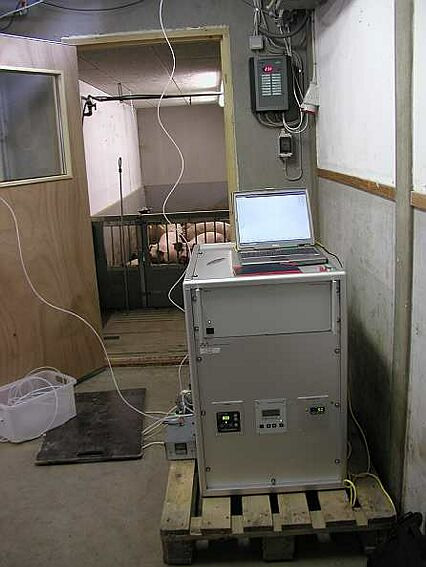
Workshop on Agricultural Air Quality Figure 1. MIMS-instrument in a pig stable
A mass spectrometer (Balzers, QMG 420) equipped with a membrane inlet consisting of a temperature controlled membrane (50 µm polydimethyl siloxane) and a stainless steel air intake was used for the measurements presented in this paper. An air pump was used to pass unfiltered air by the membrane at a flow rate of 200 ml/min providing turbulent conditions near the membrane surface, which gives the most efficient uptake of volatile compounds. Odour compounds are sampled from the air by absorption into the membrane, and because of the low pressure inside the mass spectrometer compounds diffuse through the membrane and evaporate into the ion source of the mass spectrometer. In order to monitor the efficiency of odour abatement technologies, a multiposition valve was used to multiplex between air influenced by the technology, reference air and background (clean) air. In case of a biofilter, for example, a measurement cycle consists of 1) clean air, 2) air sampled before the filter and 3) air sampled after the filter. The efficiency with respect to a certain compound is estimated from the background-subtracted signals before and after the filter, respectively. Results and Discussion
Basic Studies of MIMS Response to Odour Compounds In Figure 2, a mass spectrum obtained by sampling the headspace of manure from a Danish pig farm is presented. The sample represents a concentrated odour sample compared to typical emission levels from pig farms and is useful for evaluating which compounds contribute to the main MIMS-signals. Workshop on Agricultural Air Quality Figure 2. Assignment of MIMS-signals to odour compounds or groups of odour
compounds. The x-axis is the mass/charge ratio (m/z) of the ions formed.

It can be seen from Figure 2, that several of the major MIMS-signals can be assigned to important odour
compounds or structurally related groups of compounds. Some signals, e.g. from m/z 50 – 58 and from m/z
77 – 80 are less specific and therefore less useful for monitoring odour compounds. The composition of the
sample was confirmed by GC/MS.
There are a number of carboxylic acids present in typical samples from pig facilities. These give rise to overlapping MIMS-signals at m/z 60, 73 and 74. Therefore carboxylic acids are mainly measured as groups of compounds according to these signals. Likewise, reduced organic sulphur compounds are detected by a common signal at m/z 47 corresponding to compounds containing the CH3S- moiety, which mainly comprise methyl mercaptan, dimethyl sulphide and dimethyl disulphide. These sulphur compounds give rise to other MS-fragments that are not, however, unambiguous due to overlapping with other compounds. Other odour compounds, like skatol and indol, possess more specific MS signals. The sensitivity of MIMS is compound specific and is related to the volatility and polarity of the compound and hence its ability to be absorbed into the non-polar membrane. Carboxylic acids, for example, are highly abundant (as quantified by GC/MS) but do not give rise to the largest MIMS signals due to their high polarity. An important feature of MIMS is the linearity of the response as a function of concentration. In Figure 3, examples of calibration curves for carboxylic acids (RCOOH; the sum of carboxylic acids containing the mass spectrometric fragment with m/z 60) and p-cresol (4-methylphenol) are shown. The data in Figure 3 was obtained by injecting various amounts of a synthetic mixture of 10 important odour compounds into a Tedlar sampling bag and analyzing by MIMS. The concentration levels were selected in order to cover real-world concentration levels. P-cresol (m/z 108) Concentration (µg/m3) Concentration (µg/m3) Figure 3. Calibration curves of RCOOH (carboxylic acids) and p-cresol. The straight curves
are linear regression data.

Workshop on Agricultural Air Quality Application of MIMS for Monitoring Odour Reduction An example of results from the application of MIMS for monitoring the efficiency of a biofilter is presented in Figure 4. It appears that the efficiency of the filter towards different compounds is quite stable, whereas there is more variation regarding the efficiency towards different types of compounds. P-cresol and carboxylic acids are efficiently removed, whereas organic sulphur compounds are less reduced and with much more variability in the results. These results are not surprising since it is a prerequisite for efficient removal that the odour compounds are absorbed into the aqueous phase of the biofilter. Organic sulphur compounds, such as dimethyl sulphide, are much less water soluble than carboxylic acids or p-cresol. 02-28- 03-01- 03-02- 03-03- 03-04- 03-05- 03-06- 03-07- 03-08- 03-09- 03-10- 03-11- 03-12- Figure 4. Biofilter efficiencies towards p-cresol (black circles), RCOOH (open circles) and
reduced organic sulphur compounds (ROS; grey circles). Data from March 2005. The
efficiency is estimated from the MIMS signals before and after the filter.

Another example of application of MIMS is presented in Figure 5. In this case, the effect of cooling
ventilation air on odour emission was investigated. Two pig stable sections were compared. In one section,
the intake ventilation air was cooled in order to reduce the ventilation rate to about 50 %, whereas the other
section had a normal ventilation rate. In Figure 5, the relative effect of cooling on the emissions of
carboxylic acids and p-cresol are presented as the average diurnal variation of the measurement period of
four days. A relative effect of <1 corresponds to a reduction in the emission caused by cooling.
Workshop on Agricultural Air Quality n 4
ing o
ool 3
ffe
e
e
tiv 1
Figure 5. Average diurnal variation of the relative effect of cooling ventilation air on the
emissions of carboxylic acids (RCOOH) and p-cresol. A relative effect of <1 corresponds
to a reduction caused by cooling. Error bars represent the variation in the data.

The effect of cooling on p-cresol is relatively small with a small reduction during daytime and small
increase during nighttime in the section with cooling. Contrary to this, emission of carboxylic acids was
significantly reduced during daytime and evening, but was more strongly increased during nighttime,
although the variability in the data is quite large. The mechanisms behind these patterns cannot be
elucidated from the current work, but the results demonstrate the ability of continuous measurements to
demonstrate temporal variations that cannot be observed from single samples for olfactometric analysis or
laboratory chemical analysis.
Comparison with Olfactometry A dataset consisting of olfactometric measurements and MIMS-measurements were subject to multivariate statistical analysis in order to attempt to elucidate a statistical relationship between odour reduction observed by olfactometry and odour reduction predicted from MIMS-measurements. The analysis was based on 23 data points from 3 different types of abatement technologies and resulted in a correlation coefficient (R2) of 0.56. Although this is statistically significant (P<0.001), it is also clear that a more extensive dataset is needed for this purpose. Part of the difficulty with this approach is the inherent uncertainty associated with olfactometry. Conclusions
Membrane Inlet Mass Spectrometry (MIMS) has been tested as a technique for continuous measurements of odour compounds in or emitted from pig facilities. MIMS is able to detect a range of compounds either as individual compounds or as groups of structurally related compounds. MIMS has been demonstrated to be sufficiently robust to be used on-site and to carry out measurements unattended for extended periods of time. Examples of MIMS-measurements include long-term monitoring of the efficiency of a biofilter installed in a pig facility and monitoring the effect of cooling ventilation air on the emission of odour compounds. A tentative comparison of MIMS with olfactometry indicates a potential for predicting odour reduction from MIMS-measurements, although more data is needed to confirm this. Workshop on Agricultural Air Quality References
Blunden, J., V. P. Aneja and W. A. Lonneman. 2005. Characterization of non-methane volatile organic compounds at swine facilities in eastern North Carolina. Atmospheric Environment 39: 6707 - 6718 Hobbs, P. J., T. H. Misselbrook, and B. F. Pain. 1998. Emission rates of odorous compounds from pig slurries. Journal of the Science of Food and Agriculture 77: 341 - 348 Ketola, R. A., T. Kotiaho, M. E. Cisper, and T. M. Allen. 2002. Environmental applications of membrane introduction mass spectrometry. Journal of Mass Spectrometry 37: 457 - 476 Ketola, R. A., T. Mansikka, M. Ojala, T. Kotiaho, and R. Kostiainen. 1997. Analysis of volatile organic sulfur compounds in air by membrane inlet mass spectrometry. Analytical Chemistry 69: 4536 - 4539 Schiffman, S. S., J. L. Bennett, and J. H. Raymer. 2001. Quantification of odors and odorants from swine operations in North Carolina. Agricultural and Forest Meteorology 108: 213 - 240 Workshop on Agricultural Air Quality Understanding Biogenic GHG Emissions Using Long Path Fourier
Transform Spectroscopy (LPFTS)
N. Semmler, C.J. Ferg uson, and T.C. Hutchin 1RENTEC, Box 24, 727 Lansdowne St W, Peterborough, On K9J 6Y5 Canada al Resource Studies, Trent University, 1600 West Bank Dr, Peterborough, On K9J 7B8 Canada *Corresponding and presenting author [email protected] Abstract
Biogenic GHG emissions resulting from biological processes at the microbial level can be considerably
complex. Long Path Fourier Transform Spectroscopy (LPFTS) is a new evolving real time air pollution
monitoring technique capable of detecting multiple pollutant gas signatures by measuring the transmittance
[absorption] of light across a predetermined path.
Methodologies, protocols and algorithms developed at Trent University using LPFTS permit real time assessment of complex biogenic point source GHG as well as GHG precursor emissions. Correlation of real time observational field data obtained to known biological processes allow us to achieve a better understanding of underlying microbiology and biochemistry as well as potential "natural" mitigation strategies such as anaerobic digestion of organic [biogenic] residuals. Background
The industrialized signatories of the Kyoto Protocol have agreed to reduce their respective Greenhouse Gas (GHG) Emissions by an average of 5.2 % below 1990 emission levels. Protocol implementation has stimulated a new market where practices that reduce GHG emissions are "traded" for dollars with companies or countries that do not meet their target emission reductions. Key to equitable trading is independently verifiable determination of emissions mitigated. While industrial emissions from known processes are readily qualified as well as quantified, emissions due to biogenic processes are not always readily quantified due to the variable and complex nature of the processes themselves. Knowledge gaps exist in the areas of business as usual emissions that occur during decomposition of organic materials in uncontrolled environments such as field applied manures and controlled digestate emissions, where a complex mix of microbes are responsible for the decomposition of organic materials. If we "move" decomposition of organics into a fully controlled environment such as a digester, the substrate exits a fully enclosed vessel as stabilized digestate, emissions are voided and the organic energy potential can be harnessed in the form of biogas (65% methane and 35% CO2). The true potential to generate carbon credit trades by using anaerobic digesters for processing of surplus organic materials and surplus manures from agricultural sources have yet to be determined. The digester or biogas reactor feeds on raw manure from livestock to generate biogas and fertilizer. The biogas is harnessed and used to generate both heat and electricity using cogen technology. The GHG emission savings are two fold from this process. The first GHG saving is incurred by producing electricity from hydrocarbons that do not originate from fossil sources. Therefore every kilowatt-hour of electricity produced by using biogas as a generator fuel reduces our dependence on fossil sources and offsets a corresponding fraction of a kilowatt-hour of electricity that would otherwise have had to be generated by a process that results in ‘additional' GHG emissions. The CO2 emitted as a result of burning biogas can be considered part of a closed loop, as the CO2 generated had been ‘sequestered' previously during photosynthesis, and fed to livestock. Additional GHG emission reductions are realized due to the controlled volatization and conversion of carbon during digestion. A portion of the carbon originally present in the manure is volatized and converted to CH4 and CO2 during the digestion process and potential of digestate to emit CO2 and CH4 is reduced accordingly. N2O emissions are also potentially reduced as shown in related studies (Chatigny et al, 2003 Workshop on Agricultural Air Quality as cited in MPTWG, 2005). Since the global warming potential of CH4 and N2O are respectively 21 and 296 times that of CO2, a one-tonne reduction in N2O is equal to a 296-tonne reduction in CO2 (IPCC, 2001). Therefore there is great potential for direct mitigation of GHG's as well as generation of CO2 equivalent downstream emission credits. A significant research gap exists in the area of comparative analysis of emissions from land applied manure and digestate. Presented here is a detailed description of a measurement technique for qualitative understanding and then quantifying these reductions in the downstream emissions. Methodology
Methodology for both qualitative as well as quantitative evaluation of GHGs and precursors has been developed to better understand emission and mitigation potentials. Qualitative In order to accurately understand the GHG and precursor GHG emissions it is important to observe all the emitted constituents without interfering with the natural conditions. Natural conditions include the influence of temperature, wind, rainfall, solar radiation etc. This is accomplished by using a Long Path Fourier Transform Spectroscopy (LPFTS) technique. A Fourier Transform Spectrometer (FTS) measures the amount of light at each frequency across a predetermined spectral interval. The common spectral interval utilized here is InfraRed (IR) radiation at 400 – 4000 wave numbers (cm-1). Since molecules possess unique absorption features of IR radiation (or any radiation) the spectrometer is able to detect these constituents by monitoring the transmission of light across a predetermined path. The more molecules within the path, the more radiation absorbed within the molecules own unique region, as seen in Figure 2. The amount of absorption is mathematically represented by the following equation, which is known as the Beer-Lambert Law Where I = Intensity of light at a certain frequency after traversing path length l Io = The initial intensity of light at a certain frequency αv = The molar absorptivity of a constituent at a certain frequency C = Concentration In order to qualify differences in GHG emissions between raw and digested manure, the FTS is located between a field spread with raw manure and a field spread with digestate, as seen in Figure 1. Two mirrors are placed at the end of both fields. A broad band IR source sends light to the mirror where it is then reflected back into the spectrometer. The spectrometer measures the spectrum of light and the subsequent absorption features of every constituent present that absorbs light in this region. Figure 1: Shows an overview of the experimental configuration.

Workshop on Agricultural Air Quality The path length is the distance to the mirror and back. Measurements are taken for both fields in real time. The measurements are then divided as in Figure 2 to demonstrate the percent difference in transmitted light and the corresponding difference in concentration. Meteorological conditions are measured throughout. Ideal conditions are when the wind direction is perpendicular to the path in which the light travels. This allows us to "see"(in terms of IR absorptions) the differences in concentrations for the two fields without disturbing the natural parameters outlined above. Path lengths are typically 200 m or more, in order to provide reproducible average concentrations and minimize variabilities associated with spreading manure. It is desireable that the two fields be level and that the two light paths be at the same distance and height above ground. Quantitative In order to qu nt a ify GHG and GHG precursor emissions and associated rates the same methodology is employed as in the qualitative configuration. Only this time micrometeorological parameters such as vertical and horizontal wind direction and speed are simultaneously logged at the same time. Furthermore additional paths at different heights and horizontal positions are monitored concurrently by other FTSs. This permits reliable visualization of air movements, resulting in concentration gradients for all recorded [emitted] GHGs and GHG precursors. This data can then be used to model emission rates for all IR visible constituents. A similar micrometeorological - gradient technique has been used to calculate emission rates in previous studies using point source sample collection at different heights. It has also been compared to a SF6 tracer technique for reliability verification. The results and methodologies of this study are described in detail by Galle et al (2000). LPFTS Simulated Results
Field measurements will commence in the spring of 2006 at the Lynn Cattle Farm, located just north of London, Ontario, Canada. Topography as well as soil characteristics are documented, well known, very homogenous and therefore close to ideal at this location. In order to bench test LPFTS performance prior to field measurements, simulations were carried out. The concentration values used within the simulations were based on a study conducted by Griffith et al (1999) where elevations in atmospheric CO2, NH3 and N2O concentrations caused by land applied raw manure were simultaneously monitored using an FTS and a sample cell where the sample atmosphere was collected through Teflon tubing. The study showed that the elevation above the background concentrations for CO2, NH3 and N2O were between 0-200, 0-0.4 and 0- 0.125 ppmv respectively. In order to obtain simulated result of what is expected using the measurement configuration outlined in the methodology section, simulations of transmission measurements over a raw manure spread field and digested manure spread field were created using the FASCD3 radiative transfer model (Clough et al, 1995). The concentration values used for digestate correspond to fully digested substrate i.e. background values, which are 1.8 ppmv, 365 ppmv, 50 ppbv and 310 ppbv for CH4, CO2, NH3 and N2O respectively. In order to simulate raw manure transmission measurement values of 50 ppbv, 200 ppbv and 25 ppbv and 10 ppbv above the background value were used for CH4, CO2, NH3 and N2O respectively. These differences in concentration values fall within the limits measured in the Griffith et al (1999) study. The value for CH4 is assumed to be 50 ppbv. The two simulated measurements were then divided to give the percent difference in transmission of light at a spectral resolution of 0.125 cm-1 as shown in Figure 2. The path length used in the simulations was 200 m at a temperature of 20o C and a humidity of 40%. Figure 2 also shows a colour-coded display of the unique absorption features of CH4, CO2, NH3, and N2O. The concentrations of these constituents will be determined by matching the measured transmission difference to a simulated transmission difference. The concentrations required to make the simulation match the measured values will be equal to the concentration difference between the two fields. The plots in Figure 2 demonstrate that the above-mentioned constituents are easily detected and that lower concentration differences will also be seen. The limiting factor for lower detection limits is instrument-generated noise, which is illustrated in the error section. Workshop on Agricultural Air Quality Wavenumber (cm-1) CO Absorption Feature NH Absorption Feature N O Absorption Feature CH Absorption Feature Wavenumber (cm-1) Wavenumber (cm-1) Wavenumber (cm-1) Wavenumber (cm-1)
Figure 2: Shows the simulated difference in transmission of radiation between a raw
manure spread field and a digested manure spread field. The bottom plots show eac
the four constituents own unique absorptions.
Error Sources
Error (%)
Instrument Calibrat o Instrument Noise Cross sectional dat Total Error *
Table 1. Shows the contribution of the various error sourc
es to the to
ror. Since each
error source is independent of one another the total error is calculated by taking the
square root of the sum of the squared error sources. * This total error is based on 0.6 %
instrument noise and a 5-minute 0.125 cm-1 measurement.
LPFTS Error
The significant sources of error in LPFTS measurements can be: instrument calibration, instrument noise and in the cross sectional data used by the FASCD3 m odel Table 1 quantifies the amount of error associated with each source. Workshop on Agricultural Air Quality The instrument noise contribution varies due to length of time and spectral resolution of measurement. The noise for two complete 5-minute measurements (digested and raw manure) equals 0.5921 % peak to peak at a resolution of 0.125 cm-1. In the case where depth of the absorption feature is only 0.5% then the noise contributes 100 % error. Obviously the LPFTS method would not use such a peak. Figure 3 shows a typical absorption feature where noise would only contribute 2 %. Wavenumber (cm-1) Figure 3. Shows the agreement between the measurement and the model for a single CH4
absorption feature.
The noise value can also be improved by reprocessing the measurement at a lower resolution if the absorption feature in question does not require a high resolution to measure it accurately. Table 2 shows th various noise values fo r eac part of the spectrum under different spectral resolutions. Region (cm-1)
0.125 cm-1
0.25 cm-1

Table 2: Noise values present in the combination
of a 5-minute digestate
a d a 5-minute raw manure measurement at three different spectral resolutions.

T e error can be improved further by repeating the analysis procedure on multiple absorption features belonging to the atmospheric constituent in question. This will reduce the error by a factor of 1/sqrt(N) where N is the number of absorption features. Discussion
From the simulated and measured instrument noise results it is evident that the LPFTS m a e hnique will be able to detect the four constituents examined here at concentration differences as low as 10 ppbv. This accuracy is adequate when compared with previous measured results as seen in the Griffith et al study. Increased precision may be required during actual field measurements for digestate. This can be accomplished in several ways. The first is increa i s ng the path length used in the measurement procedure. The LPFTS measurement technique is capable of path lengths up to 400 m. This is twice the path length examined here and would effectively doubles the absorption val e for values close to zero. The second is increasing the number of absorption features used in the analysis. If a single absorption feature yields an error value of 3.8 % and 30 similar features are used to calculate the concentration of the constituent in Workshop on Agricultural Air Quality question, the actual error value would be reduced to 0.7 %. Furthermore, instrument noise can be improved by reprocessing the measurements at a lower resolution as seen in the error section of this paper. It should be noted that although only four constituents are examined here, the LPFTS measurement technique has the ability to simultaneously monitor all the emitted constituents that absorb radiation within the region being monitored. Conclusion
In order to accurately quantify CO2 equivalent credits generated by anaerobic digesters it is important to understand the downstream GHG reductions. Considering the global warming potential factors of some of the gases in question, generation of CO2 equivalent credits in this area due to the process is potentially significant. The study to date demonstrates that the use of the LPFTS measurement technique has the potential to give a qualitative picture of the GHG and precursor concentration differences between land applied digestate and raw manure emissions without disturbing any natural parameters. This can then subsequently provide the data required to quantify the emission rate of each individual gas when coordinated with micrometeorological - gradient techniques. With particular reference to manures, past emission models prioritized direct CO2, CH4, and N2O emissions. The presented LPFTS methodology will enable definition and quantification of most if not all GHG precursors as well and assist in the development of an enhanced GHG emissions model with the potential to predict digester GHG mitigation performance based on correlation between microbial rates of digestion, carbon conversion and final emissions from digestate. References
Clough, S.A., and M.J. Iacono. 1995. Line-by-line calculation of atmospheric fluxes and cooling rates, 2, Application to carbon dioxide, ozone, methane, nitrous oxide and the halocarbons, J. Geophys. Res., 106, 16,519-16,535,. Galle, B., L.Klemedtsson, B. Bergqvist, M. Ferm, K. Tornqvist, D.W.T Griffith. N. Jensen, and F. Hansen. 2000. Measurements of ammonia emissions from spreading of manure using gradient FTIR techniques. Atmospheric Environment 34 (2000) 4907 -4915. Griffith, D.W.T., and B.Galle. 1999. Flux measurements of NH3, N2O and CO2 using dual beam FTIR spectroscopy an t d he flux Gradient technique. Atmospheric Environment 34 (2000) 1087-1098. IPCC, 2001, Climate Change 2001: Mitigation. Contribution of working group I to the third assessment report of the Intergovernmental Panel on Climate Change (Houghton, J.T., Y. Ding, D.J. Griggs, M. Noguer, P.J. van der Linden, X. Dai, K. Maskel ,l and C.A Johnson (eds.), Cambridge University Press, Cambridge. Manure Processing Technical Working Group (MPTWG), 2005, Science Discussion Paper. Saskatoon, SA, Canada. October 24-25, 2005. Singh, G., O.G. Clark, and J. Leonard. 2005. Comparison of GHG emissions from a compost pile and manure stockpile. Paper 05-074. Canadian Society for Engineering in Agricultural, Food, and Biological Systems 200 An nual Meeting. Winnipeg, Manitoba, Canada The authors gratefully acknowledge Technology Early Action Measures (TEAM) for providing financial support. Workshop on Agricultural Air Quality Presence of Heavy Metals, Dioxin-like PCBs and Mercury in Fruit and
Vegetables and Assessment of Air Quality in the Catania Territory
M. Ferrante*, E. Alonzo**, R. Fallico*, F. Platania**, R. Di Mauro***, L. Valenti****, M. Fiore*, P. Di Mattia*, M.V. Brundo*, G. Oliveri Conti*, G. Carpinteri*, S. Sciacca* *Dipartimento "G.F. Ingrassia" Igiene e Sanità Pubblica, Università degli Studi di Catania, **SIAN, AUSL 3, Catania, Sicily (Italy) ***L.AG.AM., ESA, Catania, Sicily (Italy) ****SOPAT, Adrano (CT), Sicily (Italy) Abstract
The European Community has given attention to monitoring heavy metals and PCBs because they cause
different kind of pathologies. Through this study the Authors wanted to investigate some common
products, largely consumed in the provincial territory, for heavy metals, dioxin and dioxin-like PCBs,
taking into account also the different environment matrices (soil, water, air). Results have allowed a global
evaluation on contamination of fruit and vegetables which has turned out to be generalised.
Through the "11 October 2004 Recommendation" the European Community Commission has started monitoring the baseline levels of heavy metals, dioxin and dioxin-like PCBs. The attention of the European Community for heavy metals and PCBs is based on scientific evidence proving that they cause many pathologies at different levels. Moreover, for cadmium has not been excluded a cancerogenic effect, methylmercury and dioxin-like PCBs can be teratogen, nickel is cancerogenic. Very important is also, to the Authors' opinion, the concept of "ALARA" (as low as reasonably achievable); though it is strictly connected to cultivation practices, it is also well applied to fruit and vegetables whose consumption nowadays is more and more advised to the population. Based on this background the following research objectives were set: • to verify the impact of using fertilizers on the presence of heavy metals in fruit and vegetables; • to study possible correlations between use of compost and presence of dioxin-like PCBs, taking into account also the different environment matrices (soil, water, air); • to assess the presence in the aforesaid matrices of Vanadium and Selenium that seem to protect people from diabetes, renal stones and cardiac arrhythmias; to analyse air samples in order to
confirm the eventual reduction of lead in the same matrices. Methods
In each area, samples have been taken from: - fruit and vegetables of wider consumption in the provincial territory (solanaceous, cereals, leaf vegetables, grape); - soil, water and air. After samples mineralization, metals quantitative determination was carried out in atomic absorption spectroscopy. After purification and extraction (EPA) determination of PCBs and of dioxin-like PCBs has been carried out by means of GC technique in ECD. Air samples have also been analyzed through SEM with EDX. Results and Discussion
No mercury nor PCBs were found in examined samples. Other metals were most of the times present though in moderate amount. Workshop on Agricultural Air Quality Results have allowed a global evaluation of metal contamination that, even though within legal limits, turns out to be general zed. A remarkable contribution comes from the atmospheric contamination that has been carefully weigh e Conclusions
The integrated approach, that is the basic principle of the "White book" on alimentary safety, is the only winning strategy to assure more and more alimentary safety and consumers' protection; it promot s education and involvement of all alimentary chain stakeholders.

Source: http://www.umad.de/infos/woaaq2006/Posters-d-f.pdf